Dijkstra's Shortest Path Algorithm

Breadth-first search finds the shortest path by edge count in an unweighted graph. When edges carry different weights — distances, costs, travel times — the path with the fewest edges is not necessarily the cheapest or fastest.

Example: given three routes from A to D:

• A → D directly: 1 edge, weight 20
• A → B → D: 2 edges, total weight 14
• A → C → D: 2 edges, total weight 5

BFS minimises edge count, so it returns A → D (1 edge — the fewest). But A → D costs 20. The genuinely shortest path by total weight is A → C → D at cost 5 — a 2-edge route that BFS would not select, because BFS does not consider edge weights at all. Dijkstra's algorithm solves this by tracking accumulated cost rather than hop count.

Dijkstra's algorithm solves the single-source shortest path problem on weighted graphs with non-negative edge weights. Given one source vertex, it finds the shortest path from that source to every other vertex in the graph.

In AQA exams, you will not be asked to recall the steps of Dijkstra's algorithm from memory. You will be given a partially completed working table and asked to continue or complete the trace. Understanding the logic of each step — not rote recall — is what the exam tests.

The algorithm maintains a tentative distance for each vertex: the shortest distance found so far from the source. Initially, only the source has a known distance (zero); all others are set to infinity.

At each step, the algorithm:

1. Selects the unvisited vertex with the smallest current tentative distance — call it the current vertex
2. For each unvisited neighbour of the current vertex: calculates the distance from the source via the current vertex. If this is smaller than the neighbour's recorded tentative distance, updates it
3. Marks the current vertex as permanently visited — its recorded distance is now confirmed as the shortest possible

The algorithm terminates when all vertices have been permanently visited (or when the destination vertex is confirmed, if only one shortest path is needed).

Why this works — the greedy property: Once a vertex is marked permanently visited, no shorter path to it can be discovered later. This holds as long as all edge weights are non-negative. A vertex with a tentative distance of 5 cannot be reached more cheaply via a vertex with tentative distance 8, because all edges from that vertex add further non-negative weight.

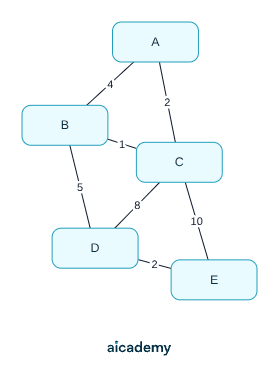
The worked trace uses this weighted undirected graph:

Edge	Weight
A–B	4
A–C	2
B–C	1
B–D	5
C–D	8
C–E	10
D–E	2

Goal: find the shortest path from A to every other vertex.

Initial state:

Vertex	A	B	C	D	E
Tentative distance	0	∞	∞	∞	∞
Visited	—	—	—	—	—

The source vertex A starts with distance 0. All others begin at infinity — meaning no path is yet known.

Tracking predecessors: alongside each tentative distance, record which vertex the update came from. This allows the shortest path to be reconstructed at the end by working backwards.

Iteration 1 — Current: A (distance 0)

Unvisited neighbours of A: B (via A = 0+4 = 4), C (via A = 0+2 = 2). Update both. Mark A visited.

Iteration 2 — Current: C (distance 2, smallest unvisited)

Unvisited neighbours of C: B (via C = 2+1 = 3 < 4 → update), D (via C = 2+8 = 10), E (via C = 2+10 = 12). Mark C visited.

Iteration 3 — Current: B (distance 3, smallest unvisited)

Unvisited neighbours of B: D (via B = 3+5 = 8 < 10 → update). Mark B visited.

Iteration 4 — Current: D (distance 8, smallest unvisited)

Unvisited neighbours of D: E (via D = 8+2 = 10 < 12 → update). Mark D visited.

Iteration 5 — Current: E (distance 10, smallest unvisited)

No unvisited neighbours. Mark E visited. All vertices visited — algorithm terminates.

After iteration	A	B	C	D	E
Initial	0	∞	∞	∞	∞
Visit A	✓	4 (via A)	2 (via A)	∞	∞
Visit C	✓	3 (via C)	✓	10 (via C)	12 (via C)
Visit B	✓	✓	✓	8 (via B)	12
Visit D	✓	✓	✓	✓	10 (via D)
Visit E	✓	✓	✓	✓	✓

The final shortest distances from A: B = 3, C = 2, D = 8, E = 10.

To find the actual path to a destination, work backwards through the predecessor chain:

Shortest path from A to E (distance 10):

• E was updated via D → predecessor of E is D
• D was updated (in iteration 3) via B → predecessor of D is B
• B was updated (in iteration 2) via C → predecessor of B is C
• C was updated (in iteration 1) via A → predecessor of C is A

Path: A → C → B → D → E (total weight: 2+1+5+2 = 10 ✓)

Check that no alternative path is shorter:

• A → B → D → E = 4+5+2 = 11
• A → C → E = 2+10 = 12
• A → C → D → E = 2+8+2 = 12

The algorithm found the optimal route.

Applications of Dijkstra's algorithm:

Domain	Use
GPS navigation	Finding the fastest route between locations on a road network
Network routing	Routing data packets via the lowest-latency path (e.g., OSPF protocol)
Logistics	Minimising delivery distances across a distribution network
Robotics	Pathfinding for autonomous movement around obstacles

Limitations:

Dijkstra's algorithm only works with non-negative edge weights. If any edge has a negative weight, the greedy guarantee breaks: a vertex marked as permanently visited could later be reached more cheaply via a path that includes negative-weight edges. A different algorithm (Bellman-Ford) is needed for negative weights, but this is not required by AQA 7517.

Additionally, Dijkstra finds shortest paths in a weighted graph. If all edge weights are equal, BFS achieves the same result more efficiently.

1. Selecting the wrong current vertex

At each step, select the unvisited vertex with the smallest current tentative distance. A common error is selecting the vertex with the smallest edge weight from the most recently visited vertex instead. Always scan all unvisited vertices and pick the globally smallest tentative distance.

2. Updating already-visited vertices

Once a vertex is marked permanently visited, its distance is final and must not be changed. Only update tentative distances for unvisited neighbours. Revisiting confirmed vertices produces incorrect results.

3. Forgetting to compare before updating

A tentative distance should only be updated if the new path is strictly shorter than the current recorded value. If the new distance equals or exceeds the existing tentative distance, make no change.

4. Misreading the predecessor chain

When reconstructing the path, work backwards from the destination using the predecessor (via) column. Students who try to trace forwards from the source often pick up incorrect branches. Write the predecessor of each vertex as you complete each row of the trace table.

5. Applying Dijkstra to unweighted graphs

Dijkstra works correctly on unweighted graphs but is unnecessarily slow. BFS achieves the same result in $O(V+E)$ time. If an exam question gives an unweighted graph, the expected algorithm is BFS, not Dijkstra.