Hash Tables and Dictionaries

A hash table (hash map) is a data structure that maps keys to values using a hash function to compute an index into an underlying array.

Key	Hash function gives index	Stored at
"Alice"	3	slot 3
"Bob"	7	slot 7
"Carol"	1	slot 1

Operations:

• insert(key, value): hash the key, store value at that index
• lookup(key): hash the key, retrieve value at that index
• delete(key): hash the key, remove value at that index

All three operations are $O(1)$ on average — this is the key advantage of hash tables over arrays and sorted lists.

A hash function takes a key and produces an integer index within the bounds of the array. A good hash function:

1. Is deterministic — same key always produces same index
2. Distributes keys uniformly across available slots
3. Is fast to compute

Simple example — hash a string by summing character codes modulo table size:

FUNCTION hashString(key, tableSize)
    total ← 0
    FOR i ← 1 TO LEN(key)
        total ← total + ASC(SUBSTRING(key, i, 1))
    NEXT i
    RETURN total MOD tableSize
ENDFUNCTION

Worked example — table size 10, key = "Ali":

• ASC('A') = 65, ASC('l') = 108, ASC('i') = 105
• total = 65 + 108 + 105 = 278
• index = 278 MOD 10 = 8

A collision occurs when two different keys hash to the same index. Collisions are inevitable for large datasets (infinitely many possible keys, finite table slots).

Chaining (separate chaining)

Each slot holds a linked list of all entries that hash to that slot. On collision, the new entry is appended to the list.

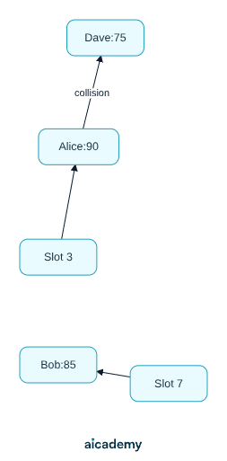
Worst case: all keys hash to one slot → $O(n)$ lookup.

Open addressing — linear probing

When a collision occurs, probe the next slot sequentially until an empty slot is found. For example, inserting "Dave" hashes to slot 3, which is occupied, so probing tries slot 4; that slot is empty, so "Dave" is stored there.

Probe sequence: index, index+1, index+2, … wrapping around the table.

Open addressing — quadratic probing

Instead of probing sequentially, the offset grows quadratically: $+1^2$, $+2^2$, $+3^2$, … So a collision at slot 3 probes slot $3+1=4$, then slot $3+4=7$, then slot $3+9=12$, and so on.

Quadratic probing reduces primary clustering (the bunching effect in linear probing where long filled runs form, slowing future insertions).

Load factor = (number of entries) / (table size). As the load factor rises, collision frequency increases and performance degrades.

Load factor	Effect
< 0.5	Low collision rate; good performance
~ 0.7	Acceptable threshold; typical rehash trigger
> 0.9	Frequent collisions; severe performance degradation

Rehashing doubles the table size and reinserts all entries when the load factor exceeds a threshold. All keys must be rehashed because the table size (the modulus) has changed.

A dictionary (also called a map or associative array) is an abstract data type that stores an unordered collection of key-value pairs where each key is unique.

Operations:

• set(key, value): add or update the value for a key
• get(key): retrieve the value associated with a key
• delete(key): remove a key-value pair
• contains(key): return True if the key exists

student_grades ← {}                // Empty dictionary

student_grades["Alice"] ← 90      // set
student_grades["Bob"]   ← 85

OUTPUT student_grades["Alice"]     // get → 90

student_grades["Alice"] ← 92      // update

IF "Bob" IN student_grades THEN   // contains
    DELETE student_grades["Bob"]   // delete
ENDIF

A dictionary is an abstract data type — the interface is defined by its operations (get, set, delete), not its implementation. The same ADT can be implemented in different ways.

AQA requires knowledge of two common dictionary implementations:

	Hash table	Binary search tree (BST)
Average lookup	$O(1)$	$O(\log n)$
Worst-case lookup	$O(n)$ (all keys collide)	$O(n)$ (degenerate/unbalanced tree)
Key ordering	Unordered	Keys stored in sorted order
Range queries	Not efficient	Efficient (in-order traversal)
Memory	Requires pre-allocated table	Dynamic; no wasted space
Best for	Fast single-key lookup	Ordered iteration or range queries

Hash table implementation: hash the key to find the index directly. Average $O(1)$.

BST implementation: store key-value pairs as BST nodes, keys determining position. Lookup traverses the tree: go left if key < current node, right if key > current node. $O(\log n)$ average.

Worked example — storing word frequencies:

freq ← {}
FOR each word IN document
    IF word IN freq THEN
        freq[word] ← freq[word] + 1
    ELSE
        freq[word] ← 1
    ENDIF
NEXT

A hash table implementation gives $O(1)$ per word; a BST implementation gives $O(\log n)$ per word but keeps words in alphabetical order if traversed in-order.

1. Claiming hash tables are always O(1)

Hash table operations are $O(1)$ on average, assuming a good hash function and low load factor. In the worst case (all keys collide to one slot), lookup is $O(n)$.

2. Confusing the dictionary ADT with its implementation

A dictionary is defined by its operations. A hash table is one implementation; a BST is another. Describing a dictionary as "a hash table" conflates the abstraction with one particular implementation.

3. Forgetting quadratic probing in open-addressing questions

AQA names both linear and quadratic probing. Linear probing uses sequential slots (+1, +2, +3, …); quadratic uses growing offsets (+1, +4, +9, …). Confusing the two or omitting quadratic loses marks.

4. Not accounting for collisions in exam traces

When tracing a hash table insertion, check whether the computed slot is already occupied. Apply the collision resolution strategy (chaining, linear probing, or quadratic probing) as specified by the question.